The Math
1: Planet-Star contrast for a Lambertian sphere
Contrast between and planet and its star (i.e. the ratio of planet flux to star flux, $F_p/F_s$) in reflected light depends on numerous factors including the size of the planet, planet-star separation, characteristics of the atmosphere, presence/absence of clouds, system geometry (phase). However as a first pass we can approximate the contrast by treating the planet as a Lambertian sphere, where apparent brightness is constant and incident starlight is reflected isotropically. Then, contrast as a function of phase ($\alpha$) is:
$$ C(\alpha) = \frac{2}{3} A_g(\lambda) \left(\frac{R_p}{r}\right)^2 \left[\frac{\sin\alpha + (\pi - \alpha)\cos\alpha}{\pi} \right]$$
where
$C(\alpha)$ is planet-star contrast
$ A_g(\lambda)$ is geometric albedo
$R_p$ is planet radius
$r$ is planet-star separation in the orbit plane ("true" separation)
And phase as a function of orbital elements is given by:
$$\alpha = \cos^{-1} \left(\sin(i) \;\times\; \sin(\theta + \omega_p)\right)$$
where
$\omega_p$ is argument of periastron
$i$ is inclination, with i=90 being edge on and i = 0,180 being face on
$\theta$ is the true anomaly with
$$\theta = 2 \tan^{-1} \left(\sqrt{\frac{1+e}{1-e}} \tan(E/2) \right)$$
where
$e$ is the eccentricity
$E$ is the eccentricity anomaly
with
$$M = E - e \sin E$$
$$M = 2\pi \frac{\Delta t}{P}$$
where
$M$ is the mean anomaly
$\Delta t$ is the time since periastron passage
$P$ is the orbital period
(see Cahoy et al. 2010 Eqn 1, Sobolev 1975)
This plot shows 100s of the nearest ($<$70 pc) known RV-detected planets in the Exoplanet Archive (as of Aug 2023), plotted as a function of separation, contrast, and phase for GMagAO-X on the GMT. For planets without inclinitation values in the Archive, we used inclination = $60^{o}$, the average inclination for a uniform half-sphere. If radius was not available in the Exoplanet Archive, we used a Mass/Radius relation; if mass was not available we used Msini. Separation is in units of $\lambda$/D, the fundamental length scale for direct imaging (1 $\lambda$/D $\approx$ FWHM of PSF core).
This plot is interactive. Hovering your mouse over each point will give the planet information. The sliders show the effect of changing the geometric albedo $A_g$, the wavelength $\lambda$, and the primary mirror size of the telescope. The default values are for observations of $A_g$ = 0.3 Lambertian spheres in $i^{\prime}$ ($\lambda$ = 800nm) with the GMT (diameter = 25.4m). The grey dashed line marks $\lambda$/D = 2, a typical inner working angle for direct imaging; planets leftward of this line will not be detectable. The red outline marks Proxima Centauri b.
2: S/N Ratios for Atmospheric Speckle Limited Observations
Get photons per sec from a model spectrum
Next convert ergs cm$^{-1}$ s$^{-1}$ cm$^{-2}$ to photons s$^{-1}$.
Energy per photon per wavelength: $$E\,[ergs] = \frac{hc}{\lambda[cm]}$$ Number of photons per wavelength: $$n_{\gamma}\left[\frac{\gamma}{cm\,s\,cm^2}\right] = \frac{F_{\lambda}(\lambda)\left[\frac{ergs}{cm\,s\,cm^2}\right]}{E\,[ergs]}$$ Then the total flux in the filter is the sum over all wavelengths of the flux times the filter transmission curve: $$\mathrm{Total \; flux} \;[\gamma \;s^{-1} cm^{-2}] = \sum(F_\lambda(\lambda)\; [\gamma \;cm^{-1} s^{-1} cm^{-2}] \times R(\lambda) \times \delta\lambda \;[cm] )$$ where $R(\lambda)$ is the filter transmission curve as a function of wavelength, and $\delta\lambda$ is the interval the spectrum is sampled in.
Now multiply by the telescope collecting area: $$\mathrm{Total \; flux} \;[\gamma \;s^{-1}] = \mathrm{Total \; flux} \;[\gamma \;s^{-1} cm^{-2}] \times \pi r^2$$ where $r$ is the radius of the primary mirror.
Done. Total flux in a filter in photons per second.
Noise in the atmospheric speckle limited regime
The noise in a single resolution element (1 $\lambda$/D) located at the planet's separation and position angle from the star ($\overrightarrow{r_p}$) can be written as: $$ \sigma^2 = \underbrace{I_{s,*} \Delta t}_\text{Star Poisson noise} \left[\underbrace{I_c + I_{as} + I_{qs}}_\text{Star halo at planet location} + \underbrace{I_{s,*}[\tau_{as}(I_{as}^2 + 2[I_c I_{as} + I_{as} I_{qs}])}_\text{Atm speckles} + \underbrace{\tau_{qs}(I_{qs}^2 + 2I_c I_{qs})]}_\text{Quasistatic speckles} \right]\;\; + \\ \underbrace{I_{p,*} \Delta t}_\text{Planet Poisson noise} \;\; + \underbrace{I_{\rm{sky}}\Delta t N_{\rm{pix}}(\lambda)}_\text{Sky background poisson noise} \;\; + \underbrace{\left(RN \frac{\Delta t}{t_{\rm{exp}}}\right)^2}_\text{Read noise} \;\; + \underbrace{I_{dc}\Delta t N_{\rm{pix}}(\lambda)}_\text{dark current} $$ where:
- $I_{s,*}/I_{p,*}$ is the peak intensity in an aperture of size $\lambda$/D centered on the Airy core without a coronagraph in photons/sec/($\lambda$/D), incorporating telescope and instrument throughput, with $I_* = I \times T \times \pi/4 \times \rm{Strehl\;Ratio}$, where $I$ is the star/planet's intensity in a given filter, $T$ is the telescope and instrument throughput, and $\pi/4$ is the amount of starlight contained in the Airy core in an aperture of size $\lambda/D$,
- $I_c$ is the fractional contribution of intensity from residual diffraction from coronagraph,
- $I_{as}$ is the contribution from atmospheric speckles,
- $I_{qs}$ is contribution from speckles caused by instrument imperfections ("quasi-static" speckles),
- $\tau_{as}$ is the average lifetime of atmospheric speckles,
- $\tau_{qs}$ is the average lifetime of quasi-static speckles,
- $I_{sky}$ is the average sky background count rate,
- RN is the read noise,
- $I_{dc}$ is the dark current count rate,
- $\Delta t$ is the observation time,
- $t_{exp}$ is the exposure time of a single frame.
- $N_{pix}$ is the number of pixels within the area of a circle of a 1 $\lambda$/D radius,
- with $A_{\rm{\lambda/D}} \rm{[mas]} = \pi r^2, r = 0.5\lambda/D,\; \lambda/D \rm{[mas]} = 0.2063 \frac{\lambda [\mu m]}{D [\rm{m}]} \times 10^{-3}$ and A$_{pix}$ = pixel side length [mas$^2$], then $N_{pix} = A_{\rm{\lambda/D}} \rm{[mas]} / A_{pix} \rm{[mas]}$.
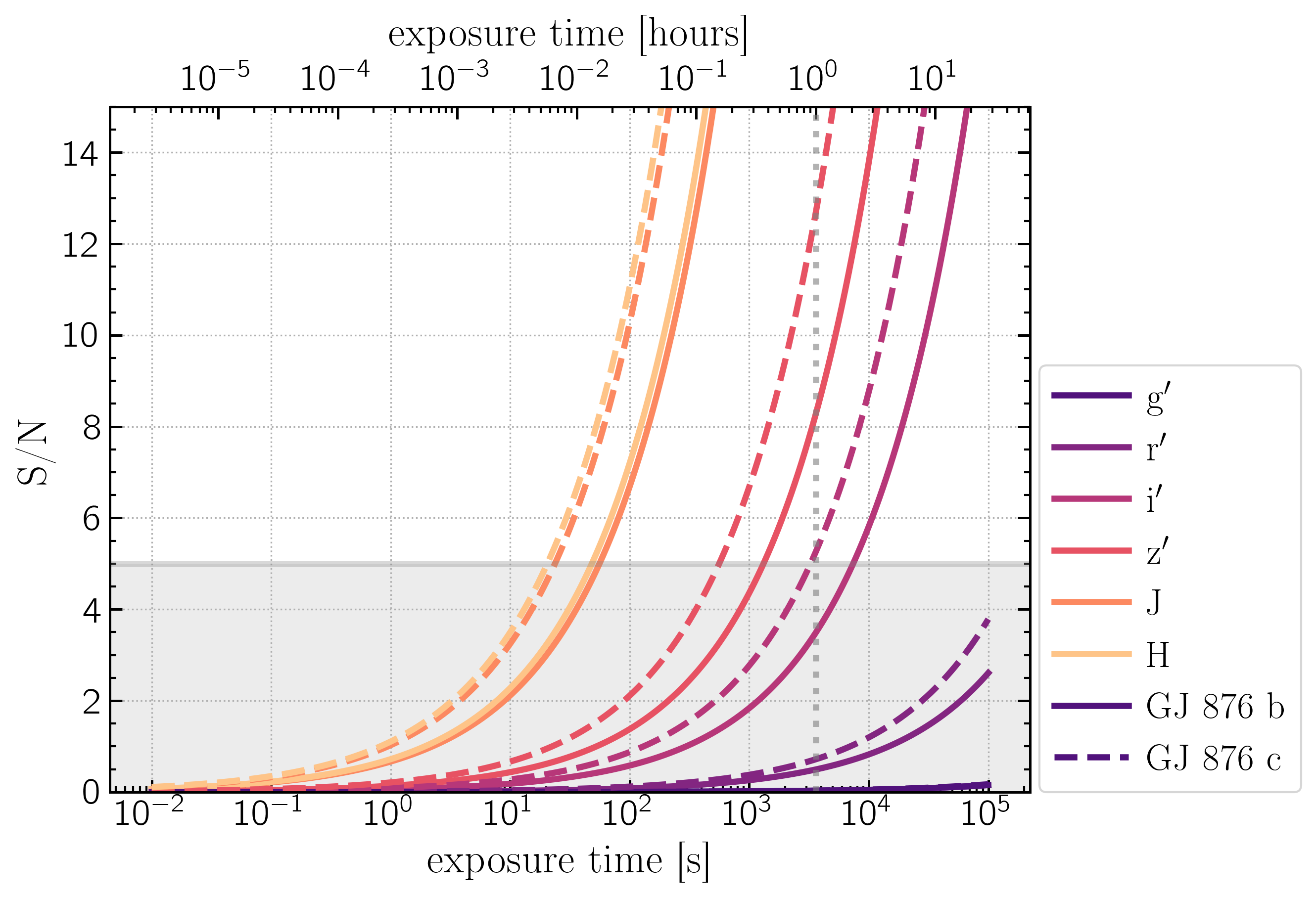
If you assume, as in Males+ 2021, that you have a perfectly functioning coronagraph and instrument such that $I_{qs}$ and $I_{c}$ terms are negligible compared to the atmospheric speckle terms, we are then in the speckle-noise limited regime. Additionally, for the purposes of these calculations I will assume that the sky, read noise, and dark current are all negligible compared to the speckles. So: $$\sigma^2 = I_* \Delta t \left[I_{as} + {I_*\tau_{as}I_{as}^2}\right]\;\; + I_p \Delta t$$ and S/N becomes: $$S/N \approx \frac{I_{p,*} \Delta t}{\sqrt{I_{s,*} \Delta t \left[I_{as} + {I_{s,*}\tau_{as}I_{as}^2}\right]\;\; + I_{p,*} \Delta t}}$$ and then: $$\Delta t = \left(\frac{S/N}{I_p}\right)^2 \left[I_{s,*} \left(I_{as} + {I_{s,*}\tau_{as}I_{as}^2}\right) + I_{p,*} \right] $$ Here is an example using ReflectX models for GJ 876 b and c at quadrature, kzz = 1e9, and fsed = 0.03:
3: Viewing phase angle given orbital elements
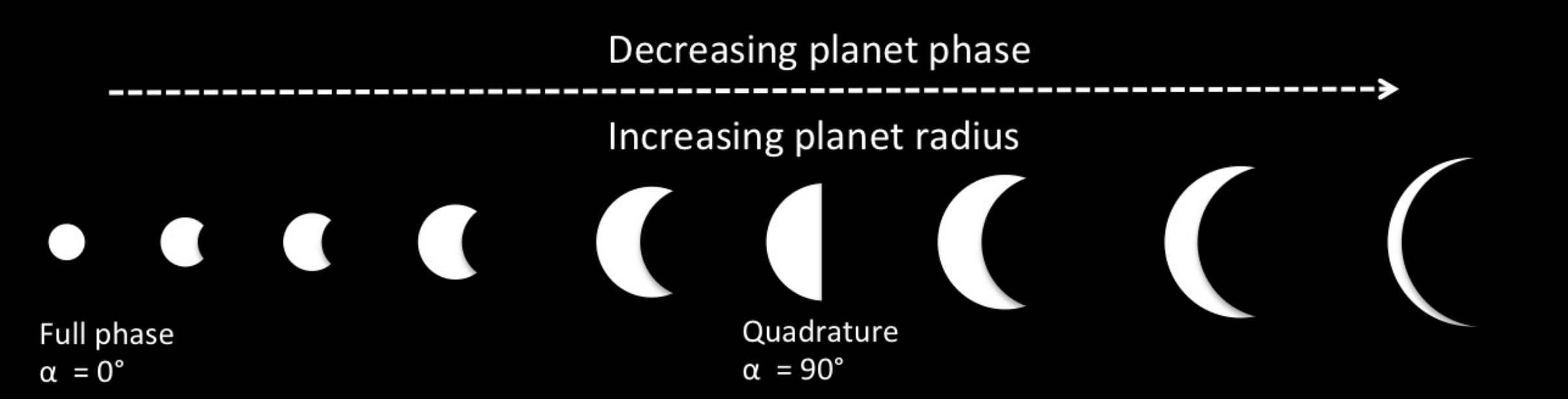
Small planets at fuller phase can yeild the same reflected flux as a larger planet at larger phase. To break the degeneracy it is necessary to know the phase or the radius a priori.
Above in Section 1 we adopted a Lambertian phase function, however this is something PICASO integrates into climate solutions, see here, and so is taken as an input into PICASO models.
Viewing phase as a function of orbital elements is given by:
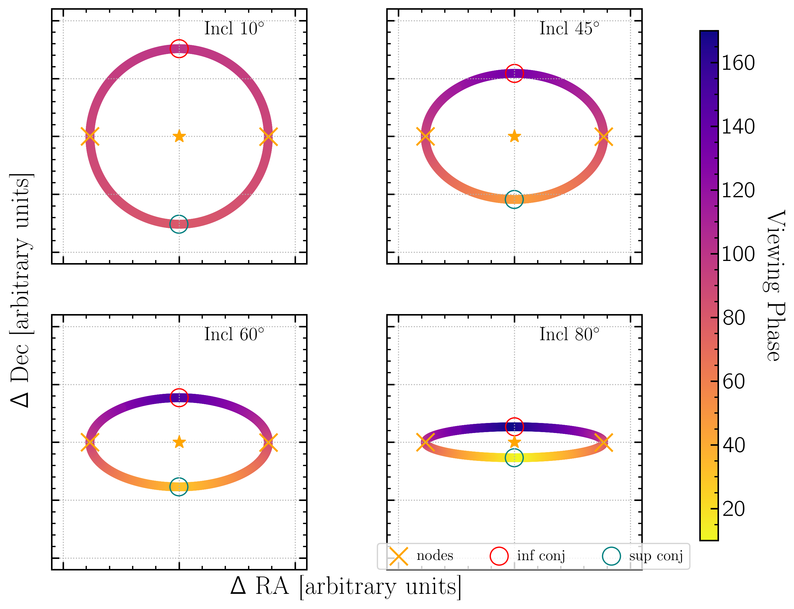
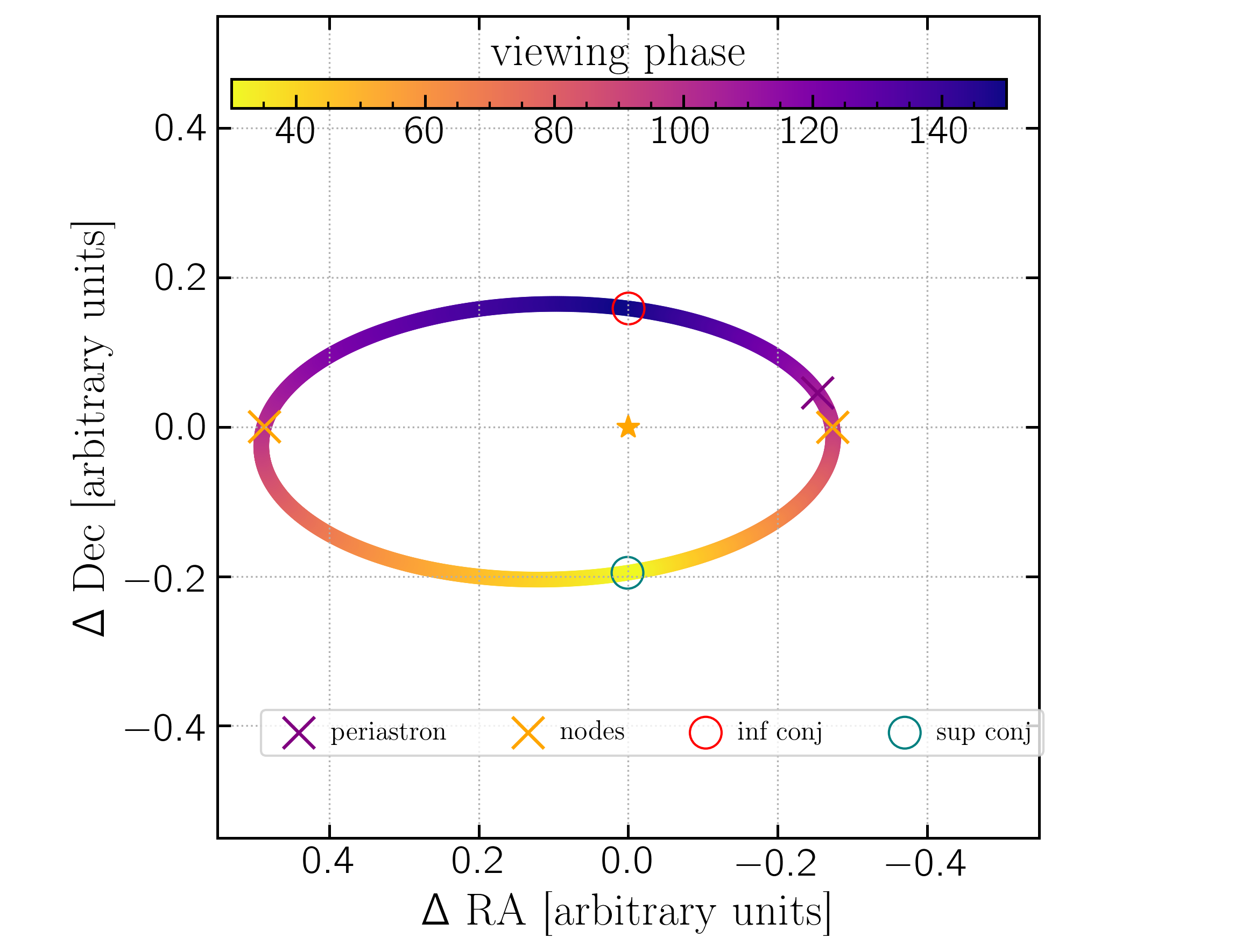
$$\alpha = \cos^{-1} \left(\sin(i) \; \sin(\phi)\right)$$ where $i$ is inclination, with i=90 being edge on and i = 0,180 being face on, and $\phi$ is an angle describing the location along the orbit in the plane of the sky.
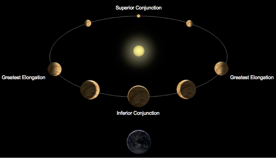
$\phi = 0$, the maximum phase or faintest, is defined at inferior conjunction -- the point when the planet passes between the star and observer (if the planet transits it will be at inferior conjunction) -- and $\phi = 180$ is superior conjunction, the minimum or brightest phase.
$$f_{\rm{inf}} = \frac{\pi}{2} - \omega$$ and for superior conjunction is
$$f_{\rm{sup}} = \frac{\pi}{2} + \omega$$
Then eccentricity anomaly at inferior conjunction is:
$$ E_{\rm{inf}} = 2 \tan^{-1} \left[ \tan(\frac{f_{\rm{inf}}}{2}) \sqrt{ \frac{1-e}{1+e}} \right]$$
And mean anomaly at inferior conjunction is:
$$M_{\rm{inf}} = E_{\rm{inf}} - e\;\sin(_{\rm{inf}})$$ With this analytical solution I ran into some trickeries with angles and greater/less than 90 deg, so I developed a code to find it numerically and plot it correctly.
                        def alphas(inc, phis):
                            '''
                            From Lovis+ 2017 sec 2.1:

                            $\cos(\alpha) = - \sin(i) \cos(\phi)$

                            where $i$ is inclination and $\phi$ is orbital phase with $\phi= 0$ at inferior conjunction

                            args:
                                inc [flt]: inclination in degrees
                                phis [arr]: array of phi values from zero to 360 in degrees

                            returns:
                                arr: array of viewing phase angles for an orbit from inferior conjunction back to
                                    inferior conjunction
                            '''
                            alphs = []
                            for phi in phis:
                                alphs.append(np.degrees(np.arccos(-np.sin(np.radians(inc)) * np.cos(np.radians(phi)))))
                            return alphs


                        def GetPhasesFromOrbit(sma,ecc,inc,argp,lon,Ms,Mp):
                            ''' Creates an array of viewing phases for an orbit in the plane of the sky to the observer with the maximum phase
                             (faintest contrast) at inferior conjunction (where planet is aligned between star and observer) and minimum phase
                             (brightest) at superior conjunction.

                            args:
                                sma [flt]: semi-major axis in au
                                ecc [flt]: eccentricity
                                inc [flt]: inclination in degrees
                                argp [flt]: argument of periastron in degrees
                                lon [flt]: longitude of ascending node in degrees
                                Ms [flt]: star mass in solar masses
                                Mp [flt]: planet mass in Jupiter masses

                            returns:
                                arr: array of viewing phases from periastron back to periastron.

                            '''
                            # Getting phases for the orbit described by the mean orbital params:
                            import astropy.units as u
                            from myastrotools.tools import keplerian_to_cartesian, keplersconstant
                            # Find the above functions here: https://github.com/logan-pearce/myastrotools/blob/2bbc284ab723d02b7a7189494fd3eabaed434ce1/myastrotools/tools.py#L2593
                            # and here: https://github.com/logan-pearce/myastrotools/blob/2bbc284ab723d02b7a7189494fd3eabaed434ce1/myastrotools/tools.py#L239
                            # Make lists to hold results:
                            xskyplane,yskyplane,zskyplane = [],[],[]
                            phase = []
                            # How many points to compute:
                            Npoints = 1000
                            # Make an array of mean anomaly:
                            meananom = np.linspace(0,2*np.pi,Npoints)
                            # Compute kepler's constant:
                            kepmain = keplersconstant(Ms*u.Msun, Mp*u.Mjup)
                            # For each orbit point:
                            for m in meananom:
                                # compute 3d projected position:
                                pos, vel, acc = keplerian_to_cartesian(sma*u.au,ecc,inc,argp,lon,m,kepmain)
                                # add to list:
                                xskyplane.append(pos[0].value)
                                yskyplane.append(pos[1].value)
                                zskyplane.append(pos[2].value)

                            ##### Getting the phases as a function of mean anom: ###########
                            ###### Loc of inf conj:
                            # Find all points with positive z -> out of sky plane:
                            towardsobsvers = np.where(np.array(zskyplane) > 0)[0]
                            # mask everything else:
                            maskarray = np.ones(Npoints) * 99999
                            maskarray[towardsobsvers] = 1
                            # mask x position:
                            xtowardsobsvers = np.array(xskyplane)*maskarray
                            # find where x position is minimized in the section of orbit towards the observer:
                            infconj_ind = np.where( np.abs(xtowardsobsvers) == min(np.abs(xtowardsobsvers)) )[0][0]
                            ###### Loc of sup conj:
                            # Do the opposite - find where x in minimized for points into the plane/away from observer
                            awayobsvers = np.where(np.array(zskyplane) < 0)[0]
                            maskarray = np.ones(Npoints) * 99999
                            maskarray[awayobsvers] = 1
                            xawayobsvers = np.array(xskyplane)*maskarray
                            supconj_ind = np.where( np.abs(xawayobsvers) == min(np.abs(xawayobsvers)) )[0][0]

                            #### Find max and min value phases for this inclination:
                            phis = np.linspace(0,180,Npoints)
                            phases = np.array(alphas(inc,phis))
                            minphase = min(phases)
                            maxphase = max(phases)
                            # Generate empty phases array:
                            phases_array = np.ones(Npoints)

                            ###### Set each side of the phases array to range from min to max phase on either side of
                            # inf/sup conjunctions:
                            if supconj_ind > infconj_ind:
                                # Set one side of the phases array to phases from max to min
                                phases_array[0:len(xskyplane[infconj_ind:supconj_ind])] = np.linspace(maxphase,minphase,
                                                                                    len(xskyplane[infconj_ind:supconj_ind]))
                                # # Set the other side to phases from min to max
                                phases_array[len(xskyplane[infconj_ind:supconj_ind]):] = np.linspace(minphase,maxphase,
                                                                                    len(xskyplane)-len(xskyplane[infconj_ind:supconj_ind]))
                                # Finally roll the array to align with the mean anomaly array:
                                phases_array = np.roll(phases_array,infconj_ind)


                            else:
                                # Set one side of the phases array to phases from min to max
                                phases_array[0:len(xskyplane[supconj_ind:infconj_ind])] = np.linspace(minphase,maxphase,
                                                                                    len(xskyplane[supconj_ind:infconj_ind]))
                                # # Set the other side to phases from max to min
                                phases_array[len(xskyplane[supconj_ind:infconj_ind]):] = np.linspace(maxphase,minphase,
                                                                                    len(xskyplane)-len(xskyplane[supconj_ind:infconj_ind]))
                                # Finally roll the array to align with the mean anomaly array:
                                phases_array = np.roll(phases_array,supconj_ind)

                            return phases_array